The Mahalanobis distance is a statistical distance which measures the distance to the mean of a distribution in multiples of the distribution’s standard deviation.
Unfortunately it cannot be used to compare the distances of a sample point to the mean of two distributions with different standard deviations. At least, if what you actually want to know is under which distribution the sample is more probable - e.g., for associating it with that distribution.
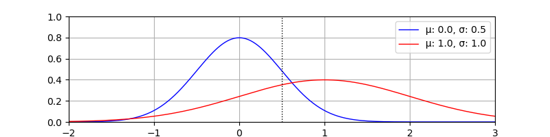
Consider the case, where you have the two normal distrbutions shown below with \(\sigma_\text{blue} = 0.5\). and \(\sigma_\text{red} = 1.0\).
Now given a sample at \(x = 0.5\) you want to know to which distribution it (more) probably belongs to. In the plot this point is shown with the vertical dottet line. Visually it is quite clear that this sample would rather belong to the blue distribution, as it has the higher probability density for \(p(x = 0.5)\).
However, when using the Mahalanobis distance, the point \(x = 0.5\) is exactly one \(\sigma_\text{blue}\) away from the blue mean, but only half a \(\sigma_\text{red}\) from the red mean.
This is because the Mahalanobis distance does not consider the normalization factor (\((2\pi)^{-\frac{k}{2}}\det(\Sigma)^{-\frac{1}{2}}\)) of the Normal distribution.
It is possible to derive a pseudo distance measure similar to the squared Mahalanobis distance work for this case, by incorporating the parts of the normalization factor that actually depends on \(x\). The other parts are the same for all distances and therefore are not needed, at least for the stated use case of deciding which one is smaller.
As for the derivation of the Mahalanobis distance, we start by taking the logarithm of the equation of the Normal distribution.
\(\ln({(2\pi)^{-\frac{k}{2}}\det(\Sigma)^{-\frac{1}{2}}e^{-\frac{1}{2}(x-\mu)^T\Sigma^{-1}(x-\mu)}})\) which can be decomposed into summands
\(\ln{(2\pi)^{-\frac{k}{2}}) + \ln(\det(\Sigma)^{-\frac{1}{2}}}) + \ln(e^{-\frac{1}{2}(x-\mu)^T\Sigma^{-1}(x-\mu)})\).
The first term is independent of \(x\), i.e. irrelevant when the only goal is to determine which distance is closer. Dropping it and simplifying the other terms leads to
\(\ln(\det(\Sigma)^{-\frac{1}{2}}) -\frac{1}{2}(x-\mu)^T\Sigma^{-1}(x-\mu)\), and
\(-\frac{1}{2}\ln(\det(\Sigma)) -\frac{1}{2}(x-\mu)^T\Sigma^{-1}(x-\mu)\).
This quantity is closely related to the probabilty. Yet the distance we seek shall be smaller for higher probability and grow for smaller probabilities. As we also don’t care about the scale, we thus multiply by \(-2\) to get the quite simple final equation
\(\ln(\det(\Sigma)) + (x-\mu)^T\Sigma^{-1}(x-\mu)\),
which is basically the squared Mahalanobis distance with an additional term reflecting the distribution’s normalization.
Note that we cannot take the square root of this anymore, as the first term can get negative and thus also the whole expression. As such this doesn’t really qualify as a proper distance measure. Anyway, it is useful for the stated use case.
In our one-dimensional example above, \(\det(\Sigma)\) is reduced to the variance, i.e. \(\sigma^2\), which shrinks the equation down to.
\(2\ln(\sigma)+\frac{(x-\mu)^2}{\sigma^2}\).
Plugging in the numbers from the example above (sample point at \(x=0.5\)) for the red distribution results in
\(2\ln(1.0)+\frac{0.25}{1} = 0 + 0.25 = 0.25\), while for the blue distribution we get
\(2\ln(0.5)+\frac{0.25}{0.25} = -1.386 + 1.0 = -0.386\).
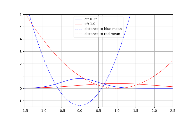
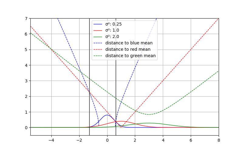
As desired, now this pseudo-distance can be compared as we would like: The “distance” to the red distributions is larger than to the blue one. The following plot shows the squared pseudo-distances. Where they are equal is marked by vertical lines. As intended these are the places where the probabilities are equal too.
In practice it allows us to find the best assignment of a data point to a set of distributions, with slightly lower computational overhead than computing the actual probabilities. Also, compared to the Mahalanobis distance, the seemingly expensive \(\det(\Sigma)\) computation can efficiently be obtained as a side-product of the inversion of \(\Sigma\). Those and the logarithm of \(\det(\Sigma)\) only have to be computed once per distribution.
Well, as long as your standard deviations (or \(\det(\Sigma)\) for multivariate distributions) are greater or equal to one, everything is fine. Otherwise, of course, you won’t get values close to the respective mean. Also, the closer to the mean, the less linearly does the distance behave, except for the case where \(\sigma = 1\), because the “normalization” part vanishes.
I am not the inventor of this method. When I learned about the method of adding \(\ln(\det(\Sigma))\) to the Mahalanobis distance I was curious, so I did the above derivation and plotting.